Modeling a Drone I: Physics

I've recently been dabbling in control systems, and have enjoyed what I've found. I decided I'd come up with a project to incentivize my learning and a quadcopter is what I landed on. I wanted to do rockets, but a drone is a little more realistic financial-wise if I ever come around to actually building the thing.

The whole thing started when I tried to see how far I could get building a physics model of a drone totally analytically in 2D. I then tried to extend what I found into 3D and had to make a few changes. Next, I decided I'd try to implement a "would-be" quadcopter flight computer, but realized it was no good unless I (a) built the quadcopter in real life or (b) created some kind of simulated environment to test the software. Since I'm much more comfortable with software I settled with (b) for now.

Here's where it all started.

Working in 2D

Imagine a coordinate system with a rigid rod extending from $(-r, r)$ on the $x$-axis. At its end points are two propellors that at any given time produce thrusts $F_l(t)$ and $F_r(t)$ perpendicular to the rod. The ultimate goal is to determine these thrusts as a function of time.

Leveling the Craft with Torque

We can measure a quantity that is the deviation from the $x$-axis as the angle $\theta$. The question becomes: how do we want our drone to react to this deviation? Qualitatively, we want the drone to set a target $\theta$ of zero and then shift the propellor thrusts to move it towards that. However, there really are an infinite amount of ways to do this. So, we need to force it to react a certain way.

One way we can do this is by considering the motion of a critically damped spring.

The above graph is the motion in one dimension of a critically damped spring through time. As you can see it “eases” into the final resting position of $x = 0$. And, if we introduce any impulse or external forces, the spring equation will attempt — in all those situations — to return to the zero point in proportion to its displacement without oscillating (the important point here).

So, if this is our desired behavior, how can we force our system to behave in this way? Well, we use this model for our $\theta$ (instead of $x$ as usual), then use an equation that relates to torque. Then, we can write our thrusts in terms of this torque to determine how the individual engines need to react. It’s a little more complicated than that, but that’s it in principle.

Let’s do this backwards.

We can write the torque of the system, in general, as

$$ \vec{\tau} = \sum \vec{r}_i\times\vec{F}_i, $$

Where $\vec{r}_i$ and $\vec{F}_i$ are the positions and forces of our engines. Since we have two we can write this as

$$ \vec{\tau} = \vec{r}\times\vec{F}_r - \vec{r}\times\vec{F}_l = \vec{r}\times(\vec{F}_r - \vec{F}_l). $$

Remember that we are working in 2D, so the direction of the torque vector will always be perpendicular to the plane. Furthermore, since the system is rigid, the forces will always be perpendicular to the displacement vectors. Thus we can write

$$ \tau = r(F_r - F_l). $$

Now, we can relate torque to the angle with a fundamental equation

$$ \tau = I\ddot{\theta} $$

where $I$ is the moment of inertia.

The moment of inertia of our system is the sum of the moment of inertias of the rod that connects the engines and the engines themselves. The moment of inertia of a rod is $m_r r^2/3$ where $m_r$ is the mass of the rod. Then, the moment of inertia of the engines are $2m_er^2$. So, $I = (m_r/3 + 2m_e)r^2$ (we’ll just keep it as $I$ for now).

We’ll come back to this equation. A spring with critical damping is modeled as Hooke’s law with a friction force, but we’re going to use torque instead of force:

$$ I\ddot{\theta} + \gamma\dot{\theta} + k\theta = 0. $$

In order for it to be critically damped we need $\gamma = 2\sqrt{Ik}$. So, substituting in $\tau$ from above, we have

$$ \tau = -2\sqrt{Ik}\dot{\theta} - k\theta, $$

where $k$ is a parameter that determines how “hard” the corrective action should be. So, if we measure $\dot{\theta}$ at every step, we can determine $\theta$ by integration. Then, using these two values, we can calculate the torque required to return the craft back to $\theta = 0$ with the desired behavior.

Determining the Thrusts

So, we can calculate the desired torque, but we still need thrust and — as you might have noticed — we have one equation and two unknowns. So, how do we find $F_l$ and $F_r$?

We can introduce another constraint we haven’t considered yet: The thrust forces should also sustain the altitude. We can write this by taking the vertical components of the forces (remember they are pointed perpendicular to the rod), adding them together, and asserting that this value is equivalent to the total weight of the craft ($w = Mg = (m_r + 2m_e)g$). Thus,

$$ Mg = \cos(\theta)(F_l + F_r). $$

So, we have our two equations:

$$ \begin{split} \tau &= r(F_r - F_l) \\ Mg &= \cos(\theta)(F_r + F_l) \end{split} $$

We can solve this by substitution, but — more generally — we can write this as a matrix equation:

$$ \begin{pmatrix} \tau \\ Mg \end{pmatrix} = \begin{pmatrix} r & -r \\ \cos(\theta) & \cos(\theta) \end{pmatrix} \begin{pmatrix} F_r \\ F_l \end{pmatrix} \implies \begin{pmatrix} r & -r \\ \cos(\theta) & \cos(\theta) \end{pmatrix}^{-1} \begin{pmatrix} \tau \\ Mg \end{pmatrix} = \begin{pmatrix} F_r \\ F_l \end{pmatrix} $$

Now we invert the matrix

$$ \begin{pmatrix} r & -r \\ \cos(\theta) & \cos(\theta) \end{pmatrix}^{-1} = \frac{1}{2r\cos(\theta)} \begin{pmatrix} \cos(\theta) & r \\ -\cos(\theta) & r \end{pmatrix} $$

to get

$$ \begin{split} \frac{Mg}{2\cos(\theta)} + \frac{\tau}{2r} &= F_r, \\ \frac{Mg}{2\cos(\theta)} - \frac{\tau}{2r} &= F_l, \end{split} $$

which is our solutions for the force.

So, we measure $\dot{\theta}$ with the IMU, integrate to keep track of $\theta$, then solve for $\tau$. Next we use $\theta$ and $\tau$ to solve for the desired thrust forces. Then we’re done!

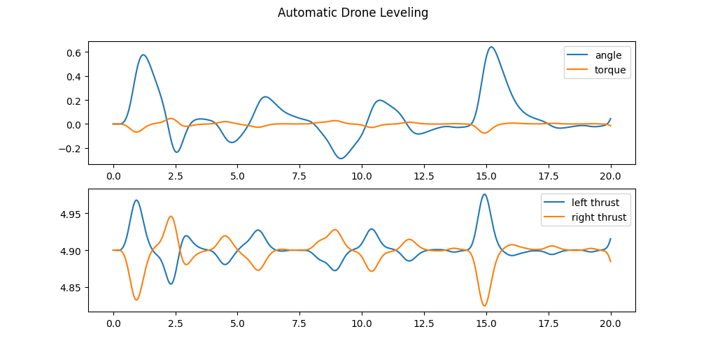
The above image is a simulation of the previously discussed logic, where there is added a random “wind” generated by Perlin noise that the torque is being tested to counter act.

Motion

In order to develop a more complete model, we must realize that the previous consideration is really a special case. Thus, we need to form more general equations that reduce to the above equations when we want the drone to be hovering.

In order to do this we will introduce another parameter $\vec{F}_d$ which is the desired net force of the craft. In order to fulfill this force in the horizontal direction, we need to introduce a new term into the torque equation and similarly for the vertical direction with the force equation.

Vertical Force

The vertical component of the desired force $F_{d\perp}$ is simple enough to add. Currently the net force is kept at zero, but we want it instead to be this force, so we just add it to the force equation

$$ \cos(\theta)(F_r + F_l) - Mg = F_{d\perp}. $$

Done.

Horizontal force

At any moment, the horizontal component of the net force on the craft is

$$ F_\parallel = \sin(\theta)(F_r + F_l) \implies F_{d\parallel} = \sin(\theta_\parallel)(F_r + F_l) $$

Currently, the spring equation we used settles to zero, but we want it to instead settle to $\theta_\parallel$, so we can determine this with

$$ \theta_\parallel = \arcsin\left(\frac{F_\parallel}{F_r + F_l}\right) $$

then alter the torque equation

$$ \tau = -2\sqrt{Ik}\dot{\theta} - k(\theta - \theta_\parallel). $$

Target Position

If we want to completely automate the motion of the drone, we can have a system that takes an input target position and the state of the drone and outputs an $\vec{F_d}$. A simple way to do this is just like we did torque, we want the critically damped spring motion to be how the displacement of the drone and its target should evolve over time.

This time we really are modeling force, so we write

$$ \vec{F}_d = 2\sqrt{Mk_d}\vec{d'} +k_d\vec{d}. $$

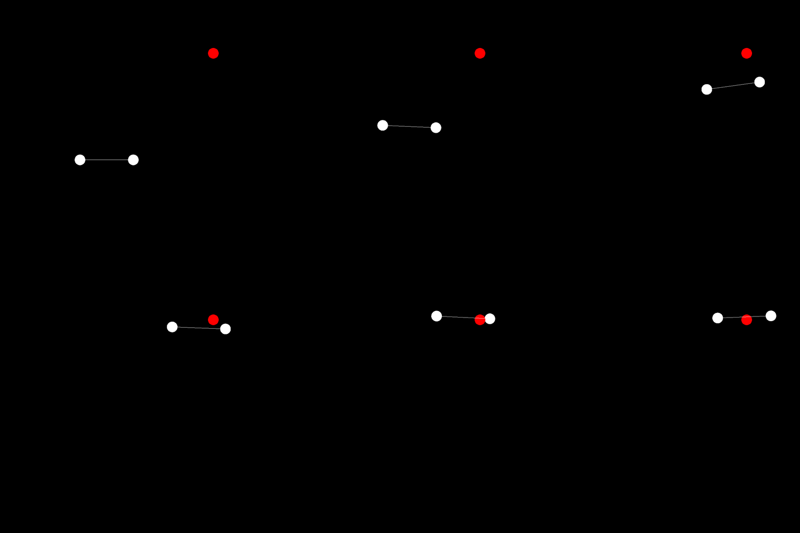
The above graphics shows all of this in action. The target position is somewhere in the top right and the drone flies up to it.

Next

The next steps are to take our model and extend it to 3D and see how far we can get.